Analysis Results from the SG registration with the Dual Sphere Superconducting Gravimeter at SAGOS (South Africa)

Jürgen Neumeyer¹⁾, Franz Barthelmes¹⁾, Ludwig Combrinck²⁾ Olaf Dierks¹⁾, Piet Fourie³

¹⁾GeoForschungZentrum Potsdam, Division 1, Telegrafenberg, 14473 Potsdam, Germany

²⁾ Hartebeesthoek Radio Astronomy Observatory, Krugersdorp , South Africa

³⁾ South African Astronomical Observatory, Sutherland , South Africa

 

1. Introduction

The installed Superconducting Gravimeter (SG) and the environmental sensors are continuously recording data since February 2000 (Neumeyer et al. 2001). These data have been preprocessed and analyzed. In detail the noise at the site, the tidal parameters, the vertical surface shift and the free oscillation of the Earth after the Peru earthquake on June 23^rd 2001 have been analyzed.

2. Calibration of the two gravity sensors

 

From both time series absolute and SG measurements the outliers and the linear trend have been removed. For determination of the calibration coefficient a linear least square fit has been performed between the Absolute Gravimeter and the SG data. 

In a second estimation the method of Fourier coefficients has been used. This method determines the amplitudes for selected frequencies from both data sets. The calibration factor is determined by the amplitude ratio obtained from Absolute Gravimeter and SG measurements at these frequencies. Both methods deliver equivalent results within the required accuracy.

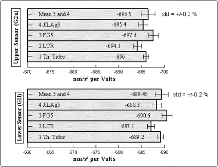
Fig. 2Calibration results of SG D037 

As the final calibration coefficient the mean between the parallel registrations of theAbsolute Gravimeters FG5 (3), JILAg5 (4) and the SG is used.The calibration factors have been determined with an standard deviation of 0.2 percent.

In a step response experiment (Van Camp et al., 1999) the time delay of both sensors has been determinedto 8.7 seconds for G1l (lower sensor)and to 7.9seconds for G2u (upper sensor). 

3. Noise at the site SAGOS

The investigation of weak gravity effects requires a low noise site. The quality of the recorded gravity data depends on the noise at the site and the noise of the instrument. The noise of the instrument is small in the inspected frequency band. 

For estimation of the noise at the site the Noise Magnitude is used (Banka and Crossley, 1999). The Noise Magnitude [NM =10* log(PSD) in dB] is calculated by the Power Spectral Density (PSD) of raw gravity data (1sec sampling rate) with a length of one month (February 2001). In figure 1 the Power Spectral Density (PSD,left axis) and the allocated Noise Magnitude (NM, right axis) are diagrammed as function of the frequency. Additionally the Noise Magnitude according to the ?New Low Noise Model? is diagrammedas graph NLNM (gray).

A comparison between the Noise Magnitude and the New Low Noise Model shows that the Noise Magnitude characterizing the quality of the site is close and even smaller as the New Low Noise Model values at frequencies below 1 mHz. This comparison shows that the site offers excellent conditions for high precision gravity measurements and the detection of weak gravity signals. In this frequency range the free oscillations of the Earth have their modes too. Therefore they can be detected very well.

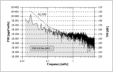
Fig 1 Noise spectra at SAGOS site

Black: Power Spectral Density (PSD) and Noise Magnitude (NM) of lower SG sensor (G1l))

Grey: New Low Noise Model (NLNM) 

4. Evaluation of gravity and environmental data

For processing of the gravity and atmospheric pressure data the Earth Tide Data Processing Package ETERNA 3.3 (Wenzel, 1996) has been used. The first high precision tidal amplitudes, amplitude factors dand phase leads khave been determined for the Sutherland site and the South African region. The tidal analysis has been performed on 18 month SG and atmospheric pressure data. The amplitude factors and the phase leads are in good agreement for both sensors of the SG. The standard deviation of the tidal analysis is ±0.7 nm/s². 

Figure 3 shows the Wahr-Dehant model (white columns) and the measured tidal amplitudes (black columns) for Sutherland. The tidal amplitudes are latitude dependent. The long periodic waves MF. MM, SSA und SA are small at Sutherland latitude of 32.38 deg South. The minimum of these waves are about at latitude 35 deg. Therefore seasonal effects (like the atmospheric pressure effect) and the polar motion (like the separation of the annual part of the polar motion from the annual tidal wave SA) can be investigated with small influence of the annual and semiannual tidal waves. The diurnal waves (maximum amplitude at latitude 0 deg)and semidiurnal waves (maximum amplitude at latitude 45 deg) can be observed well.

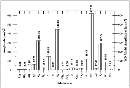
Fig. 3 Tidal amplitudes for SAGOS

White columns: Wahr-Dehant Model amplitudes

Black columns: measured amplitudes

Figure 4 shows the determined tidal parameters. For comparison the Wahr-Dehant model (white columns) and the observed amplitude factors (gray columns) are pictured. The deviations from the model can be seen clear. One reason for the deviations is the influence of the ocean loading. Therefore the ocean loading correction has been calculated for the diurnal partial tides Q1, O1, P1, K1 and the semidiurnal partial tides N2, M2, S2, K2 (Schwiderski model). The black columns show the ocean loading corrected amplitude factors. One can see that the ocean loading corrected amplitude factors come closer to the model values for the semidiurnal waves N2, M2, S2, K2 and the diurnal waves P1 and K1. For the diurnal waves Q1 and O1 the ocean loading corrected amplitude factors depart form the model values. The reason for this behavior is the ocean loading model as shown by Ducarme et. al. 2002.

The model phase is zero. Larger deviations from the model phase show the semidiurnal waves 2N2, N2, M2, L2, S2, K2 and the diurnal wave S1. The ocean corrected phase leads for the diurnal waves N2, M2, S2, K2 give a good improvement close to zero (observed values near 5 deg phase lead). The ocean correctedphase lead for the diurnal waves Q1, O1, P1, K1 become larger than the uncorrected value. 

The strong deviation (d and k) of the S1 wave to the model my be caused by the influence of the daily variations of the atmospheric pressure. Investigations for a better modeling of the atmospheric pressure influence are necessary. Furthermore the discrepancies between real measurements and the Earth tide and ocean models for the South African region have to be investigated more in detail. These discrepancies have to be abolished by improving the models and data correction for non-tidal induced gravity effects.

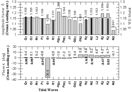
Fig 4Earth tide parameters d and k for SAGOS 

White columns: Wahr-Dehant Model parameter d

Gray columns: calculated parameters d and k

Black columns: Ocean loading corrected parameters d and k

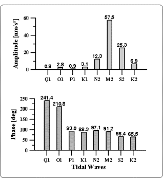
Fig.5Ocean loading effect at SAGOS for the main tidal waves

The ocean loading effect to gravity has been calculated with the program LOAD97.Figure 5 shows the correction amplitudes and the phases for the main diurnal and semidiurnal tidal waves. The most affected wave is M2 with an amplitude of 57.5 nm/s².

5. Vertical surface shift caused by Earth tides and atmospheric pressure 

Because of the elastic behaviour of the Earth the tides and changing loading on the Earth(e.g. mass redistributions in the atmosphere measured by the atmospheric pressure) cause vertical surface shift zc. This shift can be calculated by the following formula

With the elastic parameters of the Earth the Love number for elastic deformation h2 = 0.6137 and the Love number for deformation potential k2 = 0.3041, the gravimetric factor d2= 1.159 , the geocentric radius R= 6373830.451m determined with the tidal analysis and g = 9.79079 m/s² determined by absolute gravity measurements the elastic deformation coefficient for SAGOS has been determined to Dvs =-1.32 mm/µgal according to the formula

The vertical shift for SAGOS can be calculated by multiplying Dvs with the measured gravity changes Dg corrected for the atmospheric pressure effect. (Neumeyer, 1995; Kroner and Jentzsch, 1999). The atmospheric pressure correction of the gravity data has been done with the atmospheric pressure admittance coefficient apc = -2.92 µgal/hPa calculated for 

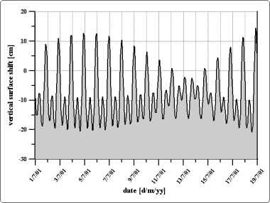
Fig. 6 Vertical surface shift caused by the Earth tides for Sutherland

SAGOS. These determined gravity changes induced by atmospheric pressure changes have been subtracted from the gravity data. Figure 6 shows the vertical surface shift zc at SAGOS for18 days in July 2001. The maximal vertical shift caused by the Earth tides and mass redistribution in the atmosphere during the time from March 27^th 2000 to August 1^st 2001 is 41.9 cm.

For separation of the atmospheric pressure influence to the vertical surface shift the Greens function method which calculatesthe attraction and deformation term separately has to be used (Sun, 1995;Neumeyer et al. 1998). With the deformation term the surface shift induced by atmospheric pressure changes can be calculated. For the Potsdam site this effect is about 2.3 cm (Neumeyer et al.,2001)

These vertical surface shift is derived from gravity measurements only. The gravity signal includes height and mass changes. It is impossible to separate mass and height changes with the gravity measurements. Therefore GPS measurements have been used to calculate the height changes for SAGOS.. 

Initial results to determine vertical displacement due to tidal forces using GPS were obtained using the GAMIT (King and Bock, 1999) software package. Additional scripts were developed to allow processing of 24 hour GPS data files using a stepped, sliding window technique. The scripts allow seamless processing over the start and end of the individual 24 hour GPS data files. Alternative processing strategies were used, varying the length of the window, the step size as well as GPS station geometry and station position constrains.No earth-tide and ocean-tide modeling were used during the processing and GPS stations were constrained horizontally but not vertically. ITRF2000 coordinates and velocities were used. The best results were obtained using a four hour window, which is stepped by 30 minutes, followed by a running average procedure to smoothen the results. This results in 48 four hour sessions per day. 

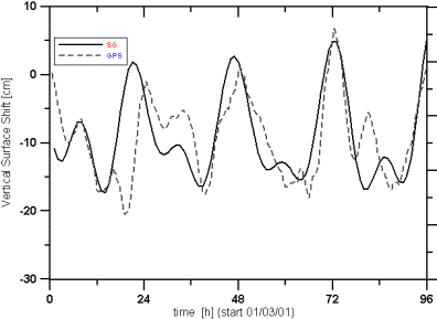
Fig. 7Vertical surface shift calculated from gravity (black line) and GPS (dashed line)

Only two GPS stations (separated by about 1000 km), the IGS stations HRAO (located at Hartebeesthoek Radio Astronomy Observatory near Pretoria)) and SUTH (located at Sutherland) were finally used. Another station towards the south (SIMO) located at Simonstown marginally degraded solutions and was therefore not included. This station (SIMO) will be included once a new station has been installed at Windhoek, Namibia, which is towards the north of Sutherland. The degrading effect is probably due to poor network geometry.Including both SIMO and the Windhoek station will improve the network geometry considerably. Improved network geometry in combination with further development of the processing scripts is expected to yield improved results. 

The first result of this calculation is shown in Figure 7. The black line shows the vertical surface shift derived from gravity measurements and the dashed line shows the first result from the GPS measurements. There is in some parts already a good agreement of both curves. 

6. Analysis of the free oscillation modes after the Peru earthquake on June 23^rd 2001 

The Earthquake near the coast of Peru (latitude 16.14S, longitude 73.312 W, depth  33 km,) on June 23^rd 2001 at 20:33:14.14 with a magnitude of 8.4 has been recorded by the mode channel of the Superconducting Gravimeter at SAGOS site.

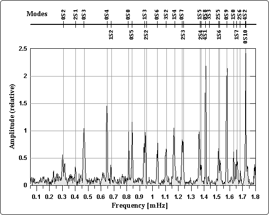
Fig 7Spheroidal free oscillation modes after the Peru earthquake on June 23^rd 2001 

The data of this Earthquake have been analyzed for detection of the free oscillation modes of the Earth. For this purpose a data set of 96 hours after the Earthquake has been corrected for atmospheric pressure. After low pass filtering (corner frequency of the filter 6 mHz) of the data the mode spectrum has been calculated by using a Hanning window (Fig. 7). Above the spectrum the different spheroidal modes are listed. Their model frequencies are at the horizontal grid lines.

The spectrum shows the model modes up to the frequency of 0S10. Especially the long periodic modes 0S3, 2S1 and 0S2 are very well marked after this Earthquake and less disturbed because of the low noise site. Compared to the results of Van Camp (1999) 2S1 and 0S2 are clear detected.

7.Acknowledgment

We thank very much Jacques Hinderer, Martine Amalvict and Bernard Luck ?Ecole et Observatoire desSciences de la Terre? Strasbourg ,France for carrying out absolute gravity measurements at SAGOS with the Absolute Gravimeter FG5 in February 2001.

We thank very much Jaakko Makinen ? Finnish Geodetic Institute? Masala, Finland for carrying out absolute gravity measurements at SAGOS with the Absolute Gravimeter JILAg5 in March 2001.

References

Banka, D., Crossley, D., (1999) Noise levels of superconducting gravimeters at seismic frequencies, Geophys. J. Int. 139, 87-97

Crossley, D., Hinderer, J., Casula, O., Francis, O., Hsu, H.T., Imanishi, Y., Jentzsch, G., Kääriäinen J., Merriam J., Meurers B., Neumeyer J., Richter B., Sato D., Shihuya K., van Dam T., (1999) Network of Superconducting Gravimeters Benefits a Number of Disciplines, EOS. Trans. Am. Geoph. Union, 80, 11, 125-126

Ducarme, B., Sun, H.-P., Xu, Q.X. (2002) New Investigations of Tidal Gravity Results from the GGp Network, submitted toMarees Terrestres Bulletin d´Informations, Brussels

Hinderer, J., Amalvict, M., Franzis, O., Mäkinen, J., (1998) On the calibration of superconducting gravimeters with the help of absolute gravity measurements, in Proc. 13^th Int. Symp. Earth Tides,

Brussels 1997, Eds.: B. Ducarme and P. Paquet,557-564

Hinderer, J., Florsch, N., Mäkinen, J., Legros, H., Faller, J. E., (1991) On the calibration of a superconducting gravimeter using absolute gravity measurements, Geophys. J. Int., 106, 491-497

King, R. W., and Bock Y., (1999) Documentation for the GAMIT GPS analysis software, Mass. Inst. of Technol., Cambridge Mass.

Kroner C., Jentzsch G., (1999) Comparison of different barometric pressure reductions for gravity data and resulting consequences. Phys. Earth Planet. Inter. 115, 205-218.

Neumeyer J. (1995) Frequency dependent atmospheric pressure correction on gravity variations by means of cross spectral analysis. Marees Terrestres Bulletin d´Informations, Bruxelles, 122, 9212-9220.
 

Neumeyer J., Barthelmes F., Wolf D. (1998) Atmospheric Pressure Correction for Gravity Data Using Different Methods. Proc. of the 13^th Int. Symp. on Earth Tides, Brussels, 1997, Eds.: B. Ducarme and P. Paquet,431-438.

Neumeyer J., Barthelmes F., Wolf D., (1999): Estimates of environmental effects in Superconducting Gravimeter data. Marees Terrestres Bulletin d'Informations, Bruxelles, 131, 10153-10159

Neumeyer, J. and Stobie B., (2000): The new Superconducting Gravimeter Site at the South African Geodynamic Observatory Sutherland (SAGOS). Cahiers du Centre Europeen de Geodynamique et de Seismologie, Volume 17,85-96.

Neumeyer J., Brinton E., Fourie P., Dittfeld H.-J., Pflug H., Ritschel B., (2001): Installation and first data analysis of the Dual Sphere Superconducting Gravimeter at the South African Geodynamic Observatory Sutherland. Journal of the Geodetic Society of Japan Vol. 47, No.1, 316-321

Neumeyer,J., Barthelmes F., Dittfeld H.-J., (2001) Ergebnisse aus einer sechsjährigen Registrierung mit dem Supraleitgravimeter am GFZ Potsdam, Zeitschrift für Vermessungswesen, Heft 1, Jg. 126, 15-22 

Sun H.-P., (1995) Static deformation and gravity changes at the Earth's surface due to the atmospheric pressure. Observatoire Royal des Belgique, Serie Geophysique Hors-Serie, Bruxelles.

Van Camp M., (1999) Measuring seismic normal modes with the GWR C021 superconducting gravimeter. Phys. Earth Planet. Inter. 116, 81-92.

Van Camp M., Wenzel H.-G., SchottP., Vauterin P., Francis O., (1999) Accurate transfer function determination for superconducting gravimeter, Geophys. Res. Lett., VOL. 27, NO. 1, 37-40.

Wenzel, H.-G., (1996) The nanogal software: Earthtide data processing package ETERNA 3.3. Marees Terrestres Bulletin d'Informations, Bruxelles, 124, 9425-9439.